You’ve got questions, I’ve got data. Cities are changing and everyone wants to know the impact. What follows is a constantly updating FAQ that helps to answer the big questions in housing economics and urbanism.

How do new market-rate apartments affect rental prices?

When new market-rate housing gets built, what happens to everyone’s rents around the build? There are two theorized effects:

• The supply effect – New buildings absorb demand, reducing pressure on rents.
• The amenity effect – New development will attract high-income households and new amenities, driving up rents.

Xiaodi Li (2019) found that when a new luxury apartment is built in NYC:

• nearby house prices fall
• nearby rents fall
• more restaurants opened up and
• low-rent units didn’t see rent hikes

Asquith, Mast, and Reed (2020) found that for 11 major cities when more high-income people move into the neighborhood after a building is completed, the increase is totally absorbed by the new building. The arrival rate to nearby units does not seem to change. Meanwhile, rents near a new building go down by about 5-7% relative to rents slightly further away or near the sites of future construction. This means that rents are lower than they would be, not that rents go down year-over-year.

For San Francisco, Kate Pennington (2021) found that new construction caused rents to fall by 2% for parcels within 100m of the building, which had the effect of reducing a renters' risk of displacement to a lower-income neighborhood by 17%. At the same time, affordable housing wasn’t found to affect rents, displacement, or gentrification. As Pennington explained it, “These findings suggest that increasing the supply of market rate housing has beneficial spillover effects for incumbent renters, reducing rents and displacement pressure while improving neighborhood quality.”

Phillips, Manville, and Lens (2021) provides a roundup of recent publications that discuss this topic.

Bratu, Harjunen, and Saarimaa (2023) studied the effects of new, centrally-located market-rate housing in the Helsinki Metropolitan Area to discover that the “supply of new market rate units triggers moving chains that quickly reach middle- and low-income neighborhoods and individuals. Thus, new market-rate construction loosens the housing market in middle- and low-income areas even in the short run. Market-rate supply is likely to improve affordability outside the sub-markets where new construction occurs and to benefit low-income people.”

How does AirBNB affect the prices of homes?

Chen, Wei, and Xie (2022) found that when AirBnb restricted landlords to only renting out a single home in NYC, San Francisco & Portland, it immediately dropped rents by \$422 a year for a median renter & home purchase cost by \$7,057.

Sophie Calder-Wang (2022) also found a price effect but went further to generate a welfare calculation. In NYC, Airbnb led to “a total transfer of \$200M/year from renters to property owners, or \$2.7bn in NPV terms.” Bluntly, though, this transfer “reflects the regulatory conundrum caused by the severe housing supply restrictions in place.” At the same time, the “welfare impact of Airbnb remains positive because it also includes the economic gains accrued to all hosts, as well as the surpluses accrued to tourists.” From a housing perspective, the increased rent burden falls most heavily on high-income, educated, and white renters.

What is rent control?

Rent control is a broad term for laws that limit rental rates in a city or state. According to common definitions:

• In NYC specifically, rent control means that a home’s rent increases incrementally and it cannot exceed a “maximum base rent” that basically just covers the landlord’s cost for upkeep of the unit. When the tenant moves out, these apartments usually convert to rent stabilization. These units are rare at about 1% of rental units) because the current tenant must have been living in the same apartment since 1971.
• Rent stabilization: This program applies to buildings constructed before 1974 that have six units or more, and covers about 44% of rental units. Rent stabilized tenants see a limited annual rent increase.
• Generally, they put a ceiling on the maximum rent that can be charged for a unit or the amount that the rent can be increased per year.
• Vacancy control or “true rent control”: In this scenario, when a tenant moves out, the landlord can only raise the rent to the limit set by a rent control board. The rent can only be raised by a limited amount each year.
• Vacancy decontrol: When a tenant moves out, the landlord can increase the rent up to whatever the market will bear. In some places, the new rent is capped at a certain percentage over the previous rent. When the new tenant is in place, he or she will only pay a limited increase per year.

What is the impact of rent control?

Ahern and Giacoletti (2022) found that the passage of rent control in St. Paul, Minnesota in 2021:

• Caused property values to fall by 6-7%, for an aggregate loss of \$1.6 billion.
• Benefited higher incomes tenants, who were more likely to be white, while the owners who lost the most had lower incomes and were more likely to be minorities.

For properties with high-income owners and low-income tenants, the transfer of wealth was close to zero. Thus, to the extent that rent control is intended to transfer wealth from high-income to low-income households, the realized impact of the law was the opposite of its intention.

Diamond McQuade, and Qian (2019) used a 1994 law change, we exploit quasi-experimental variation in the assignment of rent control in San Francisco to study its impacts on tenants and landlords. Leveraging new data tracking individuals' migration, we find rent control limits renters' mobility by 20 percent and lowers displacement from San Francisco. Landlords treated by rent control reduce rental housing supplies by 15 percent by selling to owner-occupants and redeveloping buildings. Thus, while rent control prevents displacement of incumbent renters in the short run, the lost rental housing supply likely drove up market rents in the long run, ultimately undermining the goals of the law.

What is the impact of vacancy control?

Vacancy control is generally found to keep the rates of rental increases low and people in their homes, but it doesn’t decrease overall price. It also reduces rental units and tend to increase the number of homes. See Heskin, Levine & Garrett (2007) for an analysis of four California cities or Diamond, McQuade, and Qian (2019) for an analysis of just San Francisco.

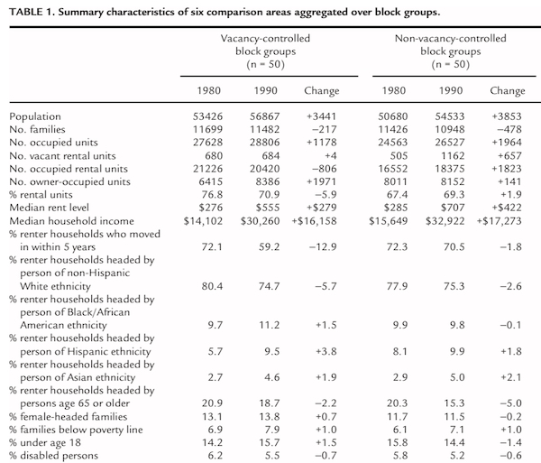
It is worth noting that vacancies are a common effect of vacancy control. Rents can only increase a limited amount every year but the apartment will often need upgrades that cost some amount of money. Landlords will wait to rent the unit until the point at which the rental rate can cover the cost of making it habitable. In other words, what you are seeing with vacancy is that the NPV of the unit is negative. It is telling.

Seth Borman had this great thread on Twitter talking about the problem.

What is the total cost of housing regulation?

The cost of regulation is high and growing for new homes. Studies released by NAHB show that regulations imposed by all levels of government account for roughly one-quarter of the sales price of a new single-family home, or about \$93,870 for a \$397,300 home. For the cost of multifamily development, more than 40% of the cost is tied up in regulations.

This paper studies the impact of state-level land-use restrictions on U.S. economic activity, focusing on how these restrictions have depressed macroeconomic activity since 2000: “We use a variety of state-level data sources, together with a general equilibrium spatial model of the United States to systematically construct a panel dataset of state-level land-use restrictions between 1950 and 2014. We show that these restrictions have generally tightened over time, particularly in California and New York. We use the model to analyze how these restrictions affect economic activity and the allocation of workers and capital across states. Counterfactual experiments show that deregulating existing urban land from 2014 regulation levels back to 1980 levels would have increased US GDP and productivity roughly to their current trend levels. California, New York, and the Mid-Atlantic region expand the most in these counterfactuals, drawing population out of the South and the Rustbelt. General equilibrium effects, particularly the reallocation of capital across states, accounts for much of these gains.”

How much of the current housing stock would be illegal to build today?

Over the past 100 years, San Francisco added numerous restrictions on housing construction. These restrictions are so severe that many existing homes would be illegal to build today. This map shows how many homes would be illegal on each parcel of lan. All told, about “54% of San Francisco homes are in buildings that would be illegal to build today.”

In New York City, approximately 40% of the buildings would be illegal to build today

How much does it cost to build an affordable home?

In San Francisco, it costs \$1.2 million to build a single affordable home, according to the Chronicle.

How does NYC’s floor-to-area ratio (FAR) impact the city?

Limits on the density of New York City’s residential housing have contributed to underdevelopment for decades. By one estimate, the FAR cap has prevented the construction of 200,000 apartments in transit rich areas of the city, enough to house almost 500,000 people. Removing this supply side limitation could be an effective tax-free measure for promoting the production of housing,” said a 2015 report from the Center for Urban Real Estate at Columbia University. It suggested the 1960s regulation is outdated, given modern HVAC and lighting systems.

Why is there so much opposition to housing?

According to some clever survey work from Nall, Elmendorf, and Oklobdzija (2022), supply skepticism is specific to housing. As they found, nearly all renters and more than half of all homeowners want future home prices & rents in their city to be lower. At the same time, only about 30%-40% believe that a influx of new homes will bring down prices. But it is not because people don’t understand supply and demand. Respondents generally gave correct answers to questions about supply shocks in other markets. In all, it seems that supply skepticism undermines renter and homeowner support for home construction.

How has COVID affected home prices?

A lot of the price growth in homes since late 2019 can be attributed to the shift to remote work. As John A. Mondragon and Johannes Wieland explain,

We show that the shift to remote work explains over one half of the 23.8 percent national house price increase over this period. Using variation in remote work exposure across U.S. metropolitan areas we estimate that an additional percentage point of remote work causes a 0.93 percent increase in house prices after controlling for negative spillovers from migration. This cross-sectional estimate combined with the aggregate shift to remote work implies that remote work raised aggregate U.S. house prices by 15.1 percent.

How have home prices affected labor supply?

Labor force participation declined significantly in 2020 and then recovered in 2021 and 2022 in a trend that has been dubbed the Great Resignation. Interestingly, the decline has been concentrated among older Americans. This is probably because increases in housing wealth drove retirements. Favilukis and Li (2023) explain, “if housing returns in 2021 would have been equal to 2019 returns, there would have been no decline in the labor force participation of older Americans.”

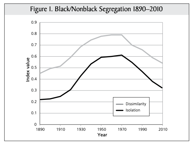
How segregated were cities in the past?

Beginning at the end of the 19th century, there was a significant rise in rental discrimination that peaks just before the Housing Act of 1969. In general, northern cities had better racial integration before zoning and redlining policies. Due to stratification based on class, poor whites and Blacks lived close to one another.

As Carolyn Adams, David Bartelt, David Elesh, Ira Goldstein explained in “Philadelphia: Neighborhoods, Division, and Conflict in a Postindustrial City” (1993):

The low levels of ethnic segregation found in the nineteenth century reflect, as in the eighteenth, the density of settlement, centralized industrial employment, and the need for almost everyone to walk to work…The Irish, Germans, and blacks, though concentrated in a few neighborhoods, were, by today’s standards, residentially integrated with the native white population.>

Glaser and Vigdor (2012) found the same:

How do racial preferences among whites and black affect neighborhoods?

One factor leading to segregation is household preferences for the racial mix of neighborhoods. Vigdor (2009) found that for whites, the ideal neighborhood having a mix of 87 percent white and 13 percent black. In contrast, the premium curve for blacks peaks at a mix of 67 percent white and 33 percent black. Because the white curve lies everywhere above the black curve, the only stable equilibrium involves racial segregation.

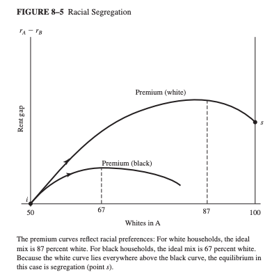
As Arthur O’Sullivan explained in Urban Economics: “What would be required to generate a stable integrated equilibrium? The slope of the black premium curve must be steeper than the white curve at the origin (50 white and 50 black households in neighborhood A). In this case, a deviation from the integrated outcome would be self-correcting because if the white population increased above 50, blacks would outbid whites for the limited number of places in the neighborhood.”

Preference also explains why black households live in neighborhoods with much lower socioeconomic status (SES) than the neighborhoods of white households with similar incomes. Many black households prefer low-SES neighborhoods with black residents to high-SES neighborhoods without black residents.

What is gentrification and what causes it?

Gentrification is typically defined as the process of a poor urban area being changed by wealthier people moving in, which then displaces current inhabitants in the process.

Quentin Brummet and Davin Reed (2019) found that,

“Gentrification modestly increases out-migration, though movers are not made observably worse off and neighborhood change is driven primarily by changes to in-migration. At the same time, many original resident adults stay and benefit from declining poverty exposure and rising house values. Children benefit from increased exposure to higher-opportunity neighborhoods, and some are more likely to attend and complete college. Our results suggest that accommodative policies, such as increasing the supply of housing in high-demand urban areas, could increase the opportunity benefits we find, reduce out-migration pressure, and promote long-term affordability.”

Yichen Su (2022) has evidence to suggest that the rising value of high-skilled workers' time contributes to the gentrification of American central cities: “I show that the increasing value of time raises the cost of commuting and exogenously increases the demand for central locations by high-skilled workers. While change in the value of time has a modest direct effect on gentrification of central cities, the effect is substantially magnified by endogenous amenity change driven by the changes in local skill mix.”

Does sprawl exist?

In a classic paper on the topic, Burchfield, Overman, Puga, and Turner (2006) found that “The extent of sprawl remained roughly unchanged between 1976 and 1992, although it varied dramatically across metropolitan areas.” Much as the standard model suggests, “Ground water availability, temperate climate, rugged terrain, decentralized employment, early public transport infrastructure, uncertainty about metropolitan growth, and unincorporated land in the urban fringe all increase sprawl.”

Why do cities exist and how does this relate to agglomeration economics?

Cities exist because they economize on costs.

Because they economize on costs, cities are places where agglomeration economies occur. Agglomeration economies are the benefits that come when firms and people locate near one another. Agglomeration economies can occur on both the production side of the equation and the consumption side of the equation.

On the production side, agglomeration economies might be technological, which make inputs more productive, or they might be pecuniary, which lowers the costs of production inputs.

Technological agglomeration economies are largely due to knowledge spillovers, both between and across firms. For more on this topic, check out Rosenthal and Strange (2004). Pecuniary agglomeration economies include lower costs for labor, lower costs for inputs (via competition), and lower costs for transportation inputs and outputs. Pecuniary agglomeration economies are a bread and butter issue, forming the basis of many core models. 

Increasingly, economists have also recognized the importance of consumption patterns to agglomeration. To summarize Glazer, Gradstein and Ranjan (2003), a consumer’s utility increases when there are different goods available, and so, the preference for variety can lead to urban agglomerations. This makes sense. People live near cities because there are things to do, places to eat, and experiences to be had.  

With access to better data, the importance of consumption is taking center stage. One recent paper of interest from Miyauchi, Nakajima, and Redding (2021) underscores the importance of local consumption. Combining smartphone data with economic census data, the authors show that non-commuting trips are frequent, more localized than commuting trips, and are strongly related to the availability of nontraded services. From here, the authors augmented a standard model to incorporate travel to work as well as this hyper local travel. Their findings are powerful. Consumption access makes a sizable contribution relative to workplace access in explaining the observed variation in residents and land prices across locations.

As a consequence, there is a substantial underestimation of the welfare gains from a transport improvement. Flemming’s work suggests that employees with lower commuting costs have much lower switching costs and climb the job ladder more effectively. Disparities in commuting costs can create big changes in outcomes.

How is the city modeled?

The benefits of agglomeration are generally modeled as increasing at a decreasing rate. Meanwhile the costs of agglomeration are typically modeled as increasing at an increasing rate. The cost of agglomeration is the pollution and hassle of living in New York City, for example. The graph below charts this concept.

The basic insight is this. The overall benefit of living in a city increases when a city goes from a lower population to a higher population, but then it reaches a maximum then starts decreasing as the city continues to grow.